Consumer Lifestyle Clustering
Recently, I have built a consumer lifestyle segmentation tool for the analytics and insight team at Mountain Equipment Co-op. The main purpose of this project is to replicate a typing tool, that has previously been developed for US consumers by a established consulting firm. This tool is leveraged to design a scalable, customer-centric marketing solution. The analysis for this tool is written in R. For further details, you can visit my Github repository.
Objectives:
- Build health lifestyle segmentation for Canadian consumers using an online survey of 2000 responses arranged by a panel provider.
- Identify clusters and interpret its meaning via descriptive statistics
- Perform pairwise comparisons among group means on profiling questions
- Future work – prototyping a lifestyle scoring tool to predict a class / segment for a new consumer
Methods
In this section, I will describe the clustering approach, its rationales and main findings.
1. Data
- The data contains a series of multi-select questions on health conditions, that respondents are currently suffer from or are concerned about preventing in the future. The answers are captured by a set of binary variables. Each represents one category in the question, in which the value 1 means the category is selected, and the value 0 means otherwise.
- It also includes additional profiling questions such as gender, age, frequency of participation in some activities, time recently spending on certain products, rate personal lifestyle goals and statements. A pruned sample of the inputs is displayed in the below table. For illustrative purposes, many columns of the dataset have been removed. Click here to view a codebook of the dataset.
| Q_AGESCREENERr1| Q_PROVINCE| Q_COMMUNITY| Q_CONDITIONr1| Q_CONDITIONr2| Q_CONDITIONr3| Q_CONDITIONr4| Q_CONDITIONr5| Q_CONDITIONr6| Q_CONDITIONr7| Q_CONDITIONr8| Q_CONDITIONr9| Q_CONDITIONr10| Q_CONDITIONr11| Q_CONDITIONr12| Q_CONDITIONr13| Q_CONDITIONr14| Q_CONDITIONr15| Q_CONDITIONr16| Q_CONDITIONr98| Q_GENDER| Q_PARENTS| Q_PREVENTIONr1| Q_PREVENTIONr2| Q_PREVENTIONr3| Q_PREVENTIONr4| Q_PREVENTIONr5| Q_PREVENTIONr6| Q_PREVENTIONr7| Q_PREVENTIONr8| Q_PREVENTIONr9| Q_PREVENTIONr10| Q_PREVENTIONr11| Q_PREVENTIONr12| Q_PREVENTIONr13| Q_PREVENTIONr14| Q_PREVENTIONr15| Q_PREVENTIONr16| Q_PREVENTIONr17| Q_PREVENTIONr98| Q_STATEMENTSr1| Q_STATEMENTSr2| Q_STATEMENTSr3| Q_STATEMENTSr4| Q_STATEMENTSr5| Q_STATEMENTSr6| Q_STATEMENTSr7| Q_STATEMENTSr8| Q_STATEMENTSr9| Q_STATEMENTSr10| Q_STATEMENTSr11| Q_STATEMENTSr12| Q_STATEMENTSr13|
|---------------:|----------:|-----------:|-------------:|-------------:|-------------:|-------------:|-------------:|-------------:|-------------:|-------------:|-------------:|--------------:|--------------:|--------------:|--------------:|--------------:|--------------:|--------------:|--------------:|--------:|---------:|--------------:|--------------:|--------------:|--------------:|--------------:|--------------:|--------------:|--------------:|--------------:|---------------:|---------------:|---------------:|---------------:|---------------:|---------------:|---------------:|---------------:|---------------:|--------------:|--------------:|--------------:|--------------:|--------------:|--------------:|--------------:|--------------:|--------------:|---------------:|---------------:|---------------:|---------------:|
|              25|          1|           3|             0|             0|             0|             0|             0|             0|             0|             0|             0|              0|              0|              0|              0|              0|              1|              0|              0|        1|         1|              0|              0|              0|              1|              0|              0|              0|              0|              0|               0|               0|               0|               0|               0|               0|               0|               0|               0|              2|              2|              2|              2|              2|              2|              2|              2|              2|               2|               2|               2|               2|
|              21|          1|           1|             1|             0|             0|             0|             0|             0|             0|             0|             0|              0|              0|              0|              0|              0|              0|              0|              0|        1|         2|              0|              0|              1|              0|              0|              0|              0|              0|              0|               0|               0|               0|               0|               0|               0|               0|               0|               0|              4|              5|              4|              5|              6|              7|              5|              5|              4|               7|               4|               4|               1|
|              24|          3|           1|             0|             0|             0|             0|             0|             0|             0|             0|             0|              0|              0|              0|              0|              0|              0|              0|              1|        2|         1|              0|              0|              0|              0|              0|              0|              0|              0|              0|               0|               0|               0|               0|               0|               0|               0|               0|               1|              5|              1|              6|              3|              1|              1|              1|              7|              6|               7|               7|               7|               1|
|              67|          9|           4|             0|             0|             0|             0|             0|             0|             0|             0|             0|              0|              0|              0|              0|              0|              0|              0|              1|        1|         2|              0|              0|              0|              0|              0|              0|              0|              0|              0|               0|               0|               0|               0|               0|               0|               0|               0|               1|              6|              3|              4|              6|              1|              3|              5|              7|              2|               4|               4|               2|               1|
|              67|          1|           5|             0|             0|             0|             0|             1|             0|             1|             0|             1|              0|              0|              0|              0|              0|              1|              0|              0|        1|         2|              1|              0|              1|              0|              0|              1|              0|              0|              1|               0|               0|               0|               0|               0|               0|               1|               0|               0|              7|              2|              7|              4|              5|              3|              2|              4|              6|               5|               7|               6|               5|
|              43|          3|           1|             0|             0|             0|             0|             0|             0|             0|             0|             0|              0|              0|              0|              0|              0|              0|              0|              1|        2|         2|              0|              0|              0|              0|              0|              0|              0|              0|              0|               0|               0|               0|               0|               0|               0|               0|               0|               1|              4|              4|              4|              4|              4|              4|              4|              4|              4|               4|               4|               4|               4|
2. Analysis:
Filter data: I remove any low-quality observation, in which a respondent speeds through the survey by giving low-effort responses, and engages in variety of other behaviors that negatively impact response quality.
Transform inputs: I regroup some health/prevention conditions into category to reduce the complexity of the inputs. This step helps to produce a cleaner interpretation of clusters in a later step. Age is dichotomized into two groups, below 58 and 58+. This threshold is based on the previous study. But other option could be explored. This coding makes all variables comparable. Note that I group any respondent, who selects both
None of the abovefor his / her health condition and prevention as a No condition cluster before proceeding to the clustering step. The reason is that one of the main interests is to find the nuance among groups who are suffering or looking to prevent varying health conditions.Select a similarity measure: In order to group observations together, I first need to define some notion of similarity between observations. Since the data contains asymmetric binary variables, I have to use a distance metric that can handle this data type. In this case, I use a metric called Gower distance. The distance is always a number between 0 (identical) and 1 (maximally dissimilar). For each binary variable, Gower distance uses one minus Jaccard’s Similarity Coefficient to calculate the dissimilarity for each binary variable. Then, the final distance is obtained as a weighted sum of these dissimilarities.
Select a clustering algorithm:
- I run both Partitioning around Medoids (PAM) and k-means algorithms for clustering. Both algorithms have linear run time and memory in terms of the number of observations assuming that the sample size is much greater than the number of variables and clusters. However, PAM is more robust to noise and outliers when compared to k-means, and it has the added benefit of having an observation serve as the exemplar for each cluster.
- Note that algorithms have similar procedure except PAM uses an observation as a cluster center (medoid), while k-means has a cluster center (centroid) defined by the mean of all observations in that cluster. Thus, I will only present the iterative steps in PAM:
- Choose k random entities to be the medoids
- Assign every entity to its closest medoid (using the custom distance matrix)
- For each cluster, identify the observation that would yield the lowest average distance to other members in the cluster. Then make this observation the new medoid.
- If at least one medoid has changed, return to the second step. Otherwise, end the algorithm.
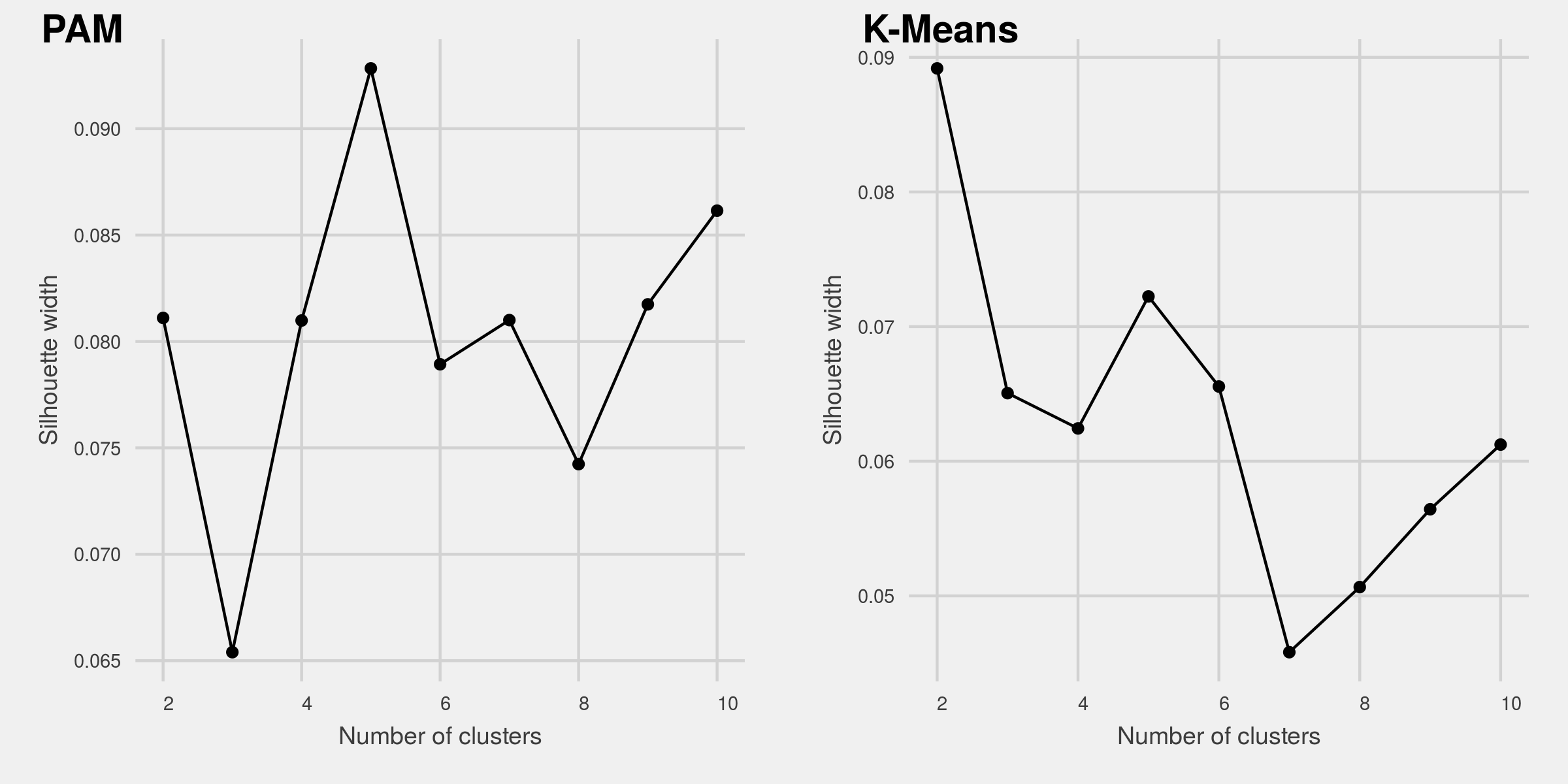
Select the number of clusters: A variety of metrics exist to help choose the number of clusters. In this analysis, I use Silhouette width as a validation metric. It is an aggregated measure of how similar an observation is to its own cluster compared its closest neighboring cluster. The metric can range from -1 to 1, where higher values are better. I then plot silhouette width for clusters ranging from 2 to 10 for both algorithms. From the Figure 1, we see that the PAM algorithm with 5 clusters yields the highest Silhouette value. On the other hand, K-Means with 2 clusters gives the highest Silhouette score.
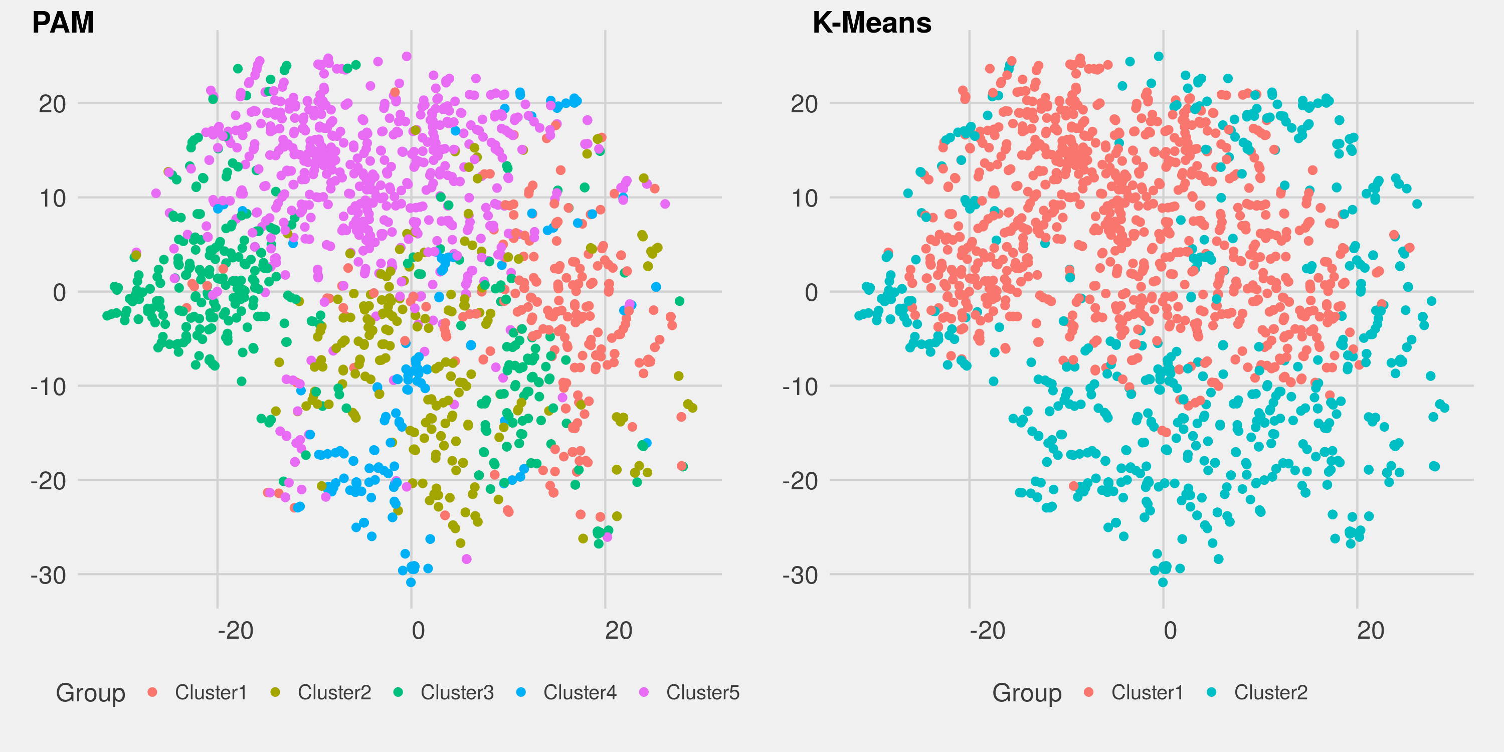
- Visualize clusters in lower dimensions: In order to see how well-separated clusters that PAM or k-means is able to detect, I employ t-distributed stochastic neighbor embedding (t-SNE) to visualize clusters in 2D. The technique tries to reduce the dimensionality of inputs, but still preserve its local structure. For further details, see the t-SNE software developed by Laurens van der Maaten.
clusterboot [in package fpc] by Christian Hennig.
* Cluster stability assessment *
Cluster method:  clara/pam
Full clustering results are given as parameter result
of the clusterboot object, which also provides further statistics
of the resampling results.
Number of resampling runs:  100

Number of clusters found in data:  5

 Clusterwise Jaccard bootstrap (omitting multiple points) mean:
[1] 0.5212346 0.4841230 0.7535759 0.6628636 0.6756281
dissolved:
[1] 53 65  4 27 23
recovered:
[1] 21 25 55 42 38
 Clusterwise Jaccard subsetting mean:
[1] 0.4776582 0.4270802 0.7189634 0.5886231 0.6485604
dissolved:
[1] 57 74  6 41 23
recovered:
[1] 13 15 40 25 31


* Cluster stability assessment *
Cluster method:  kmeans
Full clustering results are given as parameter result
of the clusterboot object, which also provides further statistics
of the resampling results.
Number of resampling runs:  100

Number of clusters found in data:  2

 Clusterwise Jaccard bootstrap (omitting multiple points) mean:
[1] 0.9707125 0.9755757
dissolved:
[1] 1 1
recovered:
[1] 99 99
 Clusterwise Jaccard subsetting mean:
[1] 0.9582220 0.9645584
dissolved:
[1] 1 1
recovered:
[1] 99 99
The assessment confirms the patterns in the t-SNE plots. The mean value of Jaccard coefficient over the bootstrap and subseting schemes suggests that two clusters found by PAM are considered unstable and can be dissolved into others. There are low certainty how observations in PAM should be grouped together. On the other hand, k-means performs better in separating observations, and capturing highly stable clusters.
- Cluster Interpretation: From the results of the above stability assessment, I decide to run the k-means algorithm with two clusters. After that, I run summary on each cluster to make interpretation. For example, it seems that Cluster 1 is mainly the people who is suffering chronic and serious conditions like high cholesterol and diabetes they want treat or prevent. They tend to be older, and often feel fatigue / lack of energy. Similar fashion can be applied to other profiling questions to infer the cluster description.
[[1]]
   age_break      COND_chronic_disease  PREV_chronic_disease
 Min.   :0.0000   Min.   :0.0000         Min.   :0.0000
 1st Qu.:0.0000   1st Qu.:0.0000         1st Qu.:1.0000
 Median :0.0000   Median :1.0000         Median :1.0000
 Mean   :0.4742   Mean   :0.6761         Mean   :0.7629
 3rd Qu.:1.0000   3rd Qu.:1.0000         3rd Qu.:1.0000
 Max.   :1.0000   Max.   :1.0000         Max.   :1.0000

omit...
3. Future work
- Applying divisive hierarchical clustering
- Employing two-step clustering when dealing with larger samples
- Prototyping a lifestyle scoring tool to predict a class / segment for a new consumer